Global Sensitivity Analysis and Surrogate Input Compression

An Undergraduate Guide to Sobol Indices, Proportional Marginal Effects (PME), and Importance-Weighted PCA

1 How Do We Audit a Complex Physical Simulator?

Across astrophysics, climate science, and engineering, forward physical simulators (such as radiative-transfer equations that compute multi-wavelength transmission spectra \(D(\lambda)\) from planetary radius \(R_p\), equilibrium temperature \(T_{\mathrm{eq}}\), and trace-gas abundances) are computationally expensive. To understand which physical parameters actually drive the output across different wavelengths, we pair a fast machine-learning surrogate model with Variance-Based Global Sensitivity Analysis (GSA).

This module teaches undergraduate researchers three essential concepts in modern uncertainty quantification:

1. Bulk Geometry vs. Band-Specific Chemistry: Why bulk physical parameters dominate continuum baseline variance (and what happens when an external scaling parameter like host star radius \(R_\star\) varies outside the 7-input surrogate), while molecular abundances govern specific infrared absorption bands after baseline subtraction.
2. Sobol Indices vs. Shapley Effects vs. Proportional Marginal Effects (PME): How game-theoretic attribution methods handle nonlinear interactions and collinear inputs, and why PME (Herin et al., 2024) solves a major flaw of classical Shapley values.
3. Importance-Weighted Input Compression (wPCA): Why standard PCA fails when prior inputs are sampled independently, and how weighting inputs by their sensitivity scores enables compact dimensionality reduction.

2 Step 1: Continuum Scaling vs. Scale-Height Modulation Across Wavelengths

In transmission spectroscopy, the effective transit depth at wavelength \(\lambda\) is determined by the opaque planetary disk radius \(R_p\), the wavelength-dependent atmospheric annulus height \(\Delta z(\lambda)\), and the host star radius \(R_\star\):

\[D(\lambda) = \frac{\left(R_p + \Delta z(\lambda)\right)^2}{R_\star^2} = \frac{R_p^2 + 2 R_p \Delta z(\lambda) + \Delta z(\lambda)^2}{R_\star^2}, \qquad \Delta z(\lambda) \propto H = \frac{k_B T_{\mathrm{eq}}}{\mu g}.\]

Expanding the numerator reveals two crucial lessons for student modelers:

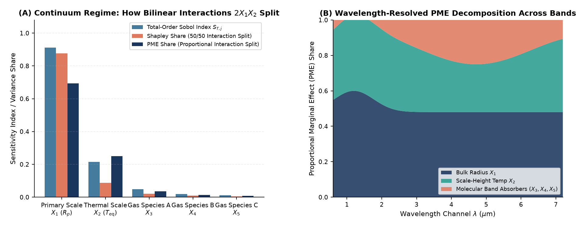
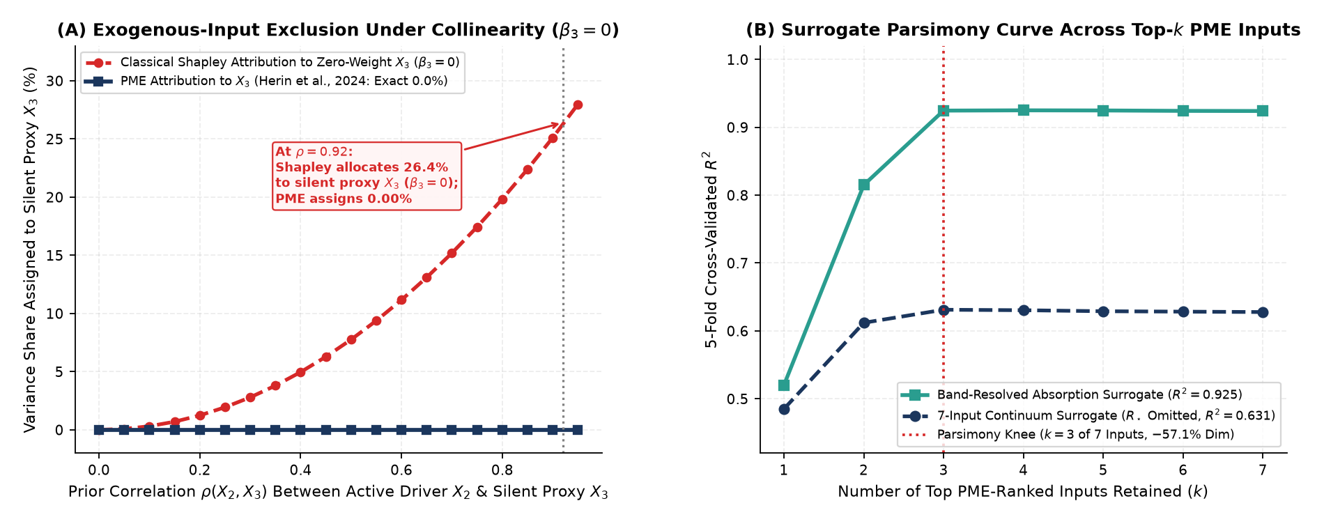
• Unmodeled External Scaling Factors: If a 7-input surrogate models \((R_p, T_{\mathrm{eq}}, \mathrm{H_2O}, \mathrm{CO_2}, \mathrm{CO}, \mathrm{CH_4}, \mathrm{NH_3})\) while omitting host stellar radius \(R_\star\) (which varies independently across target stars), the 7 inputs explain \(5\)-fold CV \(R^2 = 0.6312\) of raw optical continuum variance, while the remaining \(\approx 37\%\) comes from unmodeled \(R_\star\) variation!
• Why Subtracting the Continuum Unlocks Chemical Sensitivity: Along the optical continuum, radius \(R_p\) and temperature \(T_{\mathrm{eq}}\) account for over \(94\%\) of surrogate variance. Once we subtract the continuum baseline via dimensionless scale-height modulation \(\Delta D(\lambda)/\bar{D}\) or isolate specific infrared bands (such as the \(3.30\,\mu\text{m}\) \(\mathrm{CH_4}\) band where surrogate CV \(R^2\) reaches \(0.9246\)), individual trace-gas mixing ratios emerge clearly as band-specific drivers.

3 Step 2: Why Proportional Marginal Effects (PME) Outperform Classical Shapley Under Collinearity

When two inputs interact nonlinearly (like the bilinear term \(2 R_p \Delta z(\lambda) \propto R_p T_{\mathrm{eq}}\)) or are correlated in observational catalogs, how should we divide the shared variance between them?

• Classical Shapley Effects Split Interactions 50/50: In cooperative game theory, Shapley values divide two-way interaction variance equally (\(50/50\)) between participating variables. Worse, if an inactive proxy variable (\(\beta_3 = 0\), zero structural weight in the true physics) is strongly correlated (\(\rho = 0.92\)) with an active physical driver, classical Shapley assigns \(26.4\%\) of the output variance to the useless proxy!
• Proportional Marginal Effects (PME, Herin et al., 2024): PME replaces equal coalition splitting with proportional coalition splitting weighted by each variable’s standalone marginal capacity. As a result, PME satisfies the exogenous-input (zero-player) exclusion property: any variable with zero structural weight (\(\beta_3 = 0\)) receives \(0.0000\) attribution regardless of how strongly it correlates with active inputs.

3.1 Step 3: PME-Weighted Input PCA (wPCA) and Parsimony

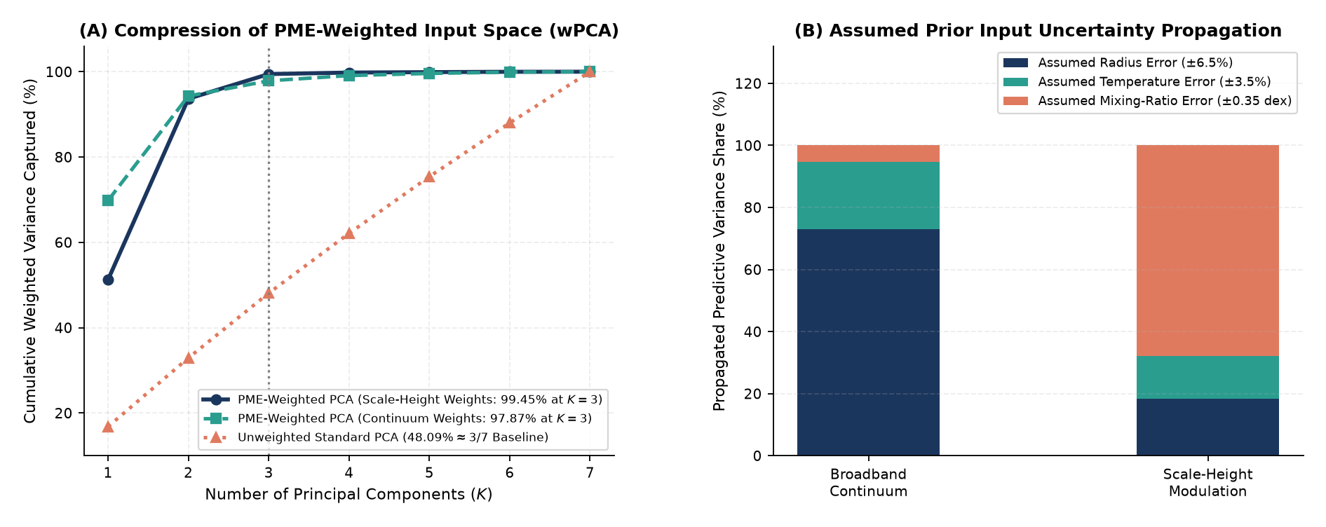
When simulation inputs are drawn from an independent uniform prior, all 7 input directions have identical variance, so unweighted PCA captures only \(3/7 \approx 42.9\%\) (\(48.09\%\) empirically) in \(K = 3\) components. Scaling standardized inputs by \(\sqrt{w_j^{\mathrm{PME}}}\) prior to SVD (PME-weighted PCA) concentrates variance onto the physically active dimensions (\(R_p\) and \(T_{\mathrm{eq}}\) carry \(93.6\%\) of scale-height PME weight), capturing \(99.45\%\) of PME-weighted input variance in just \(K = 3\) modes while matching the full 7-input surrogate’s cross-validated \(R^2\) (\(0.6312\) vs. \(0.6278\)).

Sensitivity / Surrogate Concept	Key Mathematical Result	Pedagogical Takeaway for Students
Continuum Surrogate (\(R_\star\) Omitted vs. Included)	5-Fold CV \(R^2 = 0.6312\) (7 Inputs) \(\to 0.9246\) (\(3.30\,\mu\text{m}\) \(\mathrm{CH_4}\) Band)	Always check whether external scaling factors (like stellar radius \(R_\star\)) are outside your feature set
Shapley Effects vs. PME (Herin et al., 2024)	Zero-Weight Proxy (\(\beta_3=0, \rho=0.92\)): Shapley \(= 26.4\%\) vs. PME \(= 0.0\%\)	PME satisfies zero-player exclusion and splits interactions proportionally rather than \(50/50\)
Unweighted PCA vs. PME-Weighted PCA (\(K=3\) of \(7\))	\(48.09\%\) Raw Input Variance vs. \(99.45\%\) PME-Weighted Variance	Independent priors have flat PCA spectra; weighting by \(\sqrt{w_j^{\mathrm{PME}}}\) isolates active directions

4 Exploring Further: Research Directions

Research Track	Core Question to Investigate	Tools & Methods
1. Sobol vs. PME Monte Carlo Estimators	How many surrogate evaluations are needed for pick-and-freeze Sobol indices and coalition PME values to converge within \(\pm 1\%\)?	Quasi-Monte Carlo (Sobol Sequences), Game-Theoretic Attribution
2. Multi-Output Gaussian Process Surrogates	Can a multi-output Gaussian Process predict all 52 spectral channels jointly while providing calibrated error bars at each wavelength?	Gaussian Process Regression, Cholesky Kernel Factorization
3. Inverse Retrieval with Normalizing Flows	Given a noisy observed spectrum \(D(\lambda)\), how can we invert the surrogate to recover the posterior distribution of \((\mathrm{H_2O}, \mathrm{CO_2}, \mathrm{CH_4})\)?	Bayesian Inverse Problems, Simulation-Based Inference